beta-kde: Boundary-Corrected Kernel Density Estimation
![]()
![]()
![]()
![]()
Fast, finite-sample boundary correction for data strictly bounded in [0, 1].
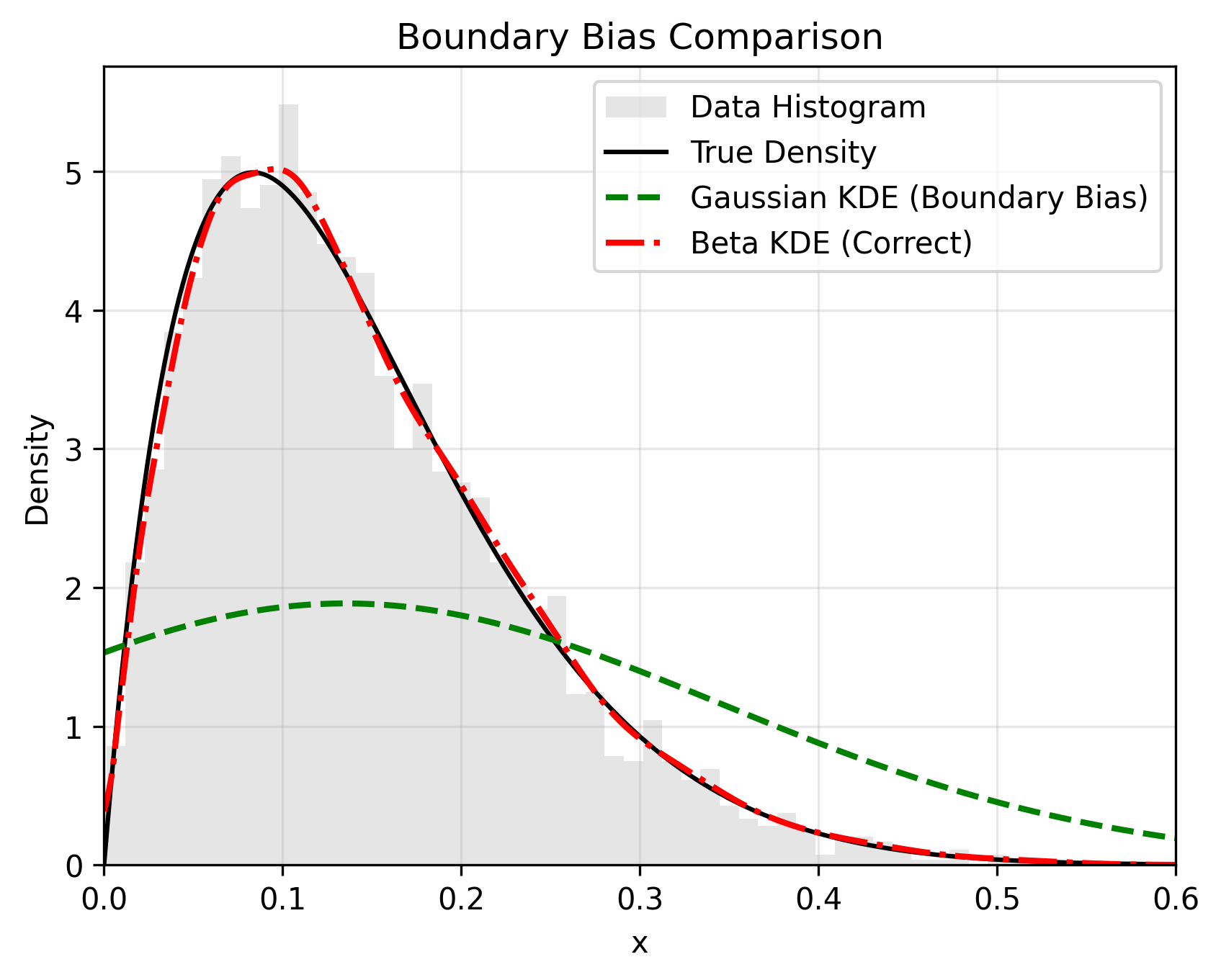
beta-kde is a Scikit-learn compatible library for Kernel Density Estimation (KDE) using the Beta kernel approach (Chen, 1999). It fixes the Boundary Bias problem inherent in standard Gaussian KDEs, where probability mass "leaks" past the edges of the data (e.g., below 0 or above 1).
📊 The Problem vs. The Solution
Standard KDEs smooth data blindly, ignoring bounds. beta-kde uses asymmetric Beta kernels that naturally adapt their shape near boundaries to prevent leakage.
🚀 Key Features
- Boundary Correction: Zero leakage. Probability mass stays strictly within the defined bounds.
- Fast Bandwidth Selection: Implements the Beta Reference Rule, a closed-form \(\mathcal{O}(1)\) selector.
It matches the accuracy of expensive Cross-Validation but is orders of magnitude faster.
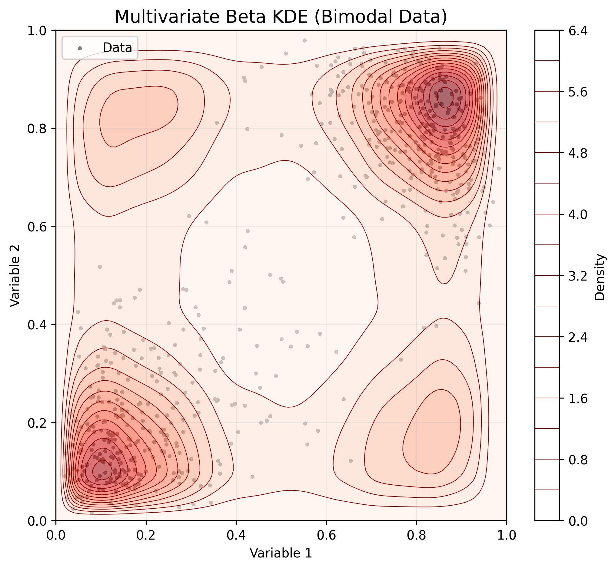
* Multivariate Support: Models multivariate bounded data using a Non-Parametric Beta Copula.
* Scikit-learn API: Drop-in replacement for KernelDensity. Fully compatible with GridSearchCV, Pipeline, and cross_val_score.
📦 Installation
pip install beta-kde
⚡ Quick Start
💡 See the Tutorial Notebook for detailed examples, including visualization and classification. 1. Univariate Data (The Standard Case) BetaKDE enforces Scikit-learn's 2D input standard (n_samples, n_features).
import numpy as np
from beta_kde import BetaKDE
import matplotlib.pyplot as plt

# 1. Generate bounded data (e.g., ratios or probabilities)
np.random.seed(42)
X = np.random.beta(2, 5, size=(100, 1))  # Must be 2D column vector

# 2. Fit the estimator
# 'beta-reference' is the fast, default rule-of-thumb from the paper
kde = BetaKDE(bandwidth='beta-reference', bounds=(0, 1))
kde.fit(X)

print(f"Selected Bandwidth: {kde.bandwidth_:.4f}")

# 3. Score samples
# Use normalized=True to get exact log-likelihoods (integrates to 1.0).
# Default is False for speed (returns raw kernel density values).
log_density = kde.score_samples(np.array([[0.1], [0.5], [0.9]]), normalized=True)

# 4. Plotting convenience
fig, ax = kde.plot()
plt.show()
- Multivariate Data (Copula)
For multidimensional data, BetaKDE fits marginals independently and models dependence using a Copula.
# Generate correlated 2D data
X_2d = np.random.rand(200, 2)

# Fit (automatically uses Copula for n_features > 1)
kde_multi = BetaKDE(bandwidth='beta-reference')
kde_multi.fit(X_2d)

# Returns log-likelihood of the joint distribution
scores = kde_multi.score_samples(X_2d)

# Plotting convenience (in the multi-variate case, this plots the marginal densities)
fig, ax = kde.plot()
plt.show()
3. Scikit-learn Compatibility (e.g. Hyperparameter Tuning)
beta-kde is a fully compliant Scikit-learn estimator. You can use it in Pipelines or with GridSearchCV to find the optimal bandwidth.
Note: The estimator automatically handles normalization during scoring to ensure valid statistical comparisons.
from sklearn.model_selection import GridSearchCV

# Define a grid of bandwidths to test
param_grid = {
    'bandwidth': [0.01, 0.05, 0.1, 'beta-reference']
}

# Run Grid Search
# n_jobs=-1 is recommended to parallelize the numerical integration
grid = GridSearchCV(
    BetaKDE(),
    param_grid,
    cv=5,
    n_jobs=-1
)

grid.fit(X)

print(f"Best Bandwidth: {grid.best_params_['bandwidth']}")
print(f"Best Log-Likelihood: {grid.best_score_:.4f}")
⚡ Performance & Normalization
Unlike Gaussian KDEs, Beta KDEs do not integrate to 1.0 analytically. Normalization requires numerical integration, which can be computationally expensive. beta-kde handles this smartly: * Lazy Loading: fit(X) is fast and does not compute the normalization constant. * On-Demand: The integral is computed and cached only when you strictly need it (e.g., calling kde.score(X) or kde.pdf(X, normalized=True)). * Flexible Scoring: * score_samples(X, normalized=False) (Default): Fast. Best for clustering, relative density comparisons, or plotting shape. * score(X): Accurate. Always returns the normalized total log-likelihood. Safe for use in GridSearchCV.
🆚 Why use beta-kde?
If your data represents percentages, probabilities, or physical constraints (e.g., \(x \in [0, 1]\)), standard KDEs are mathematically incorrect at the edges.
| Feature | sklearn.neighbors.KernelDensity |
beta-kde |
|---|---|---|
| Kernel | Gaussian (Symmetric) | Beta (Asymmetric) |
| Boundary Handling | Biased (Leaks mass < 0) | Correct (Strictly \(\ge 0\)) |
| Bandwidth Selection | Gaussian Reference Rule | Beta Reference Rule |
| Multivariate | Symmetric Gaussian Blob | Flexible Non-Parametric Copula |
| Speed (Prediction) | Fast (Tree-based) | Moderate (Exact summation) |
⚠️ Important Usage Notes
- Strict Input Shapes: Input X must be 2D. Use X.reshape(-1, 1) for 1D arrays. This constraint prevents accidental application of univariate estimators to multivariate data.
- Computational Complexity: This is an exact kernel method.
- Raw density (normalized=False) is fast.
- Exact probabilities (normalized=True) require a one-time integration cost per fitted model.
- Recommended for datasets with \(N < 50,000\).
- Bounds: You must specify bounds if your data is not in \([0, 1]\). The estimator handles scaling internally.
📚 References
- Chen, S. X. (1999). Beta kernel estimators for density functions. Computational Statistics & Data Analysis, 31(2), 131-145.
License
BSD 3-Clause License